Objectives

1. To develop Partial Least Squares (PLS) models using the plsregress function in MATLAB.
   
2. To evaluate and compare the predictive accuracies of PLS models for different input excitation patterns and sampling periods.
   
3. To implement PLS models as soft sensors for predicting distillate and bottom product impurities.

Problem Statement

Distillation columns are complex multivariable systems where direct measurement of quality variables such as distillate impurity ($y_1$) and bottom impurity ($y_2$) is often difficult or expensive. Instead, quality prediction can be achieved through soft sensors based on easily measured process variables.

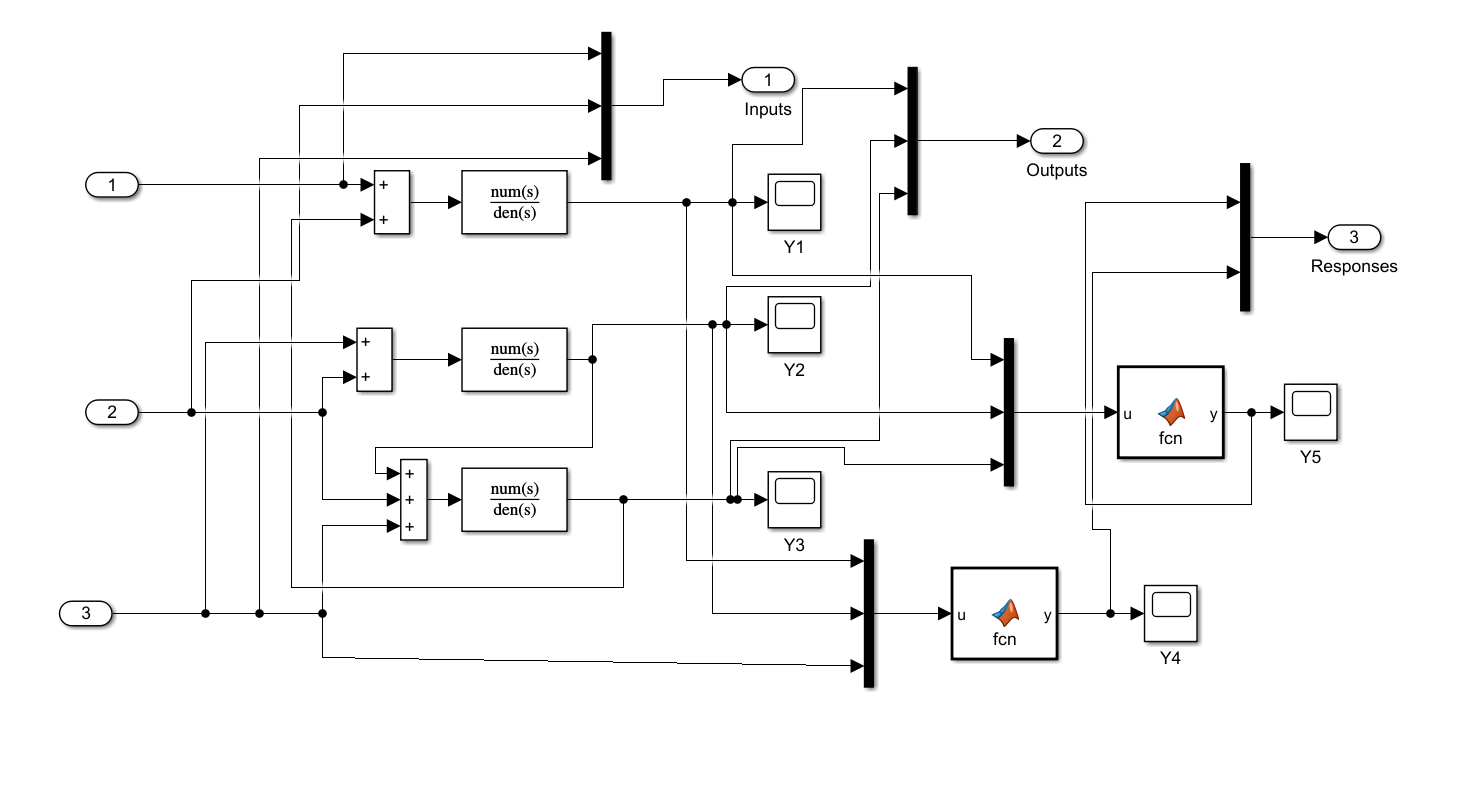
The process considered in this lab is represented by the Simulink model. The model has the following structure:

• Inputs (manipulated variables):
  • $u_1$: Feed flow rate
    
  • $u_2$: Reflux flow rate
    
  • $u_3$: Steam flow rate to the reboiler
• Measured states (secondary variables):
  • $x_1$: Tray temperature 1
    
  • $x_2$: Tray temperature 2
    
  • $x_3$: Column pressure
• Outputs (quality variables, difficult to measure):
  • $y_1$: Distillate impurity
    
  • $y_2$: Bottom impurity

Figure 1: Distillation process: distillate impurity y₁ and bottom product y₂.

Your task is to develop PLS regression models that use the available input and state variables to predict $y_1$ and $y_2$. These PLS models will serve as soft sensors, providing real-time estimates of impurities for control and monitoring.

Methodology

1. Data Generation

   • Generate datasets from the Simulink model under different input excitation schemes:
     • Uniform random signals for $u_1$, $u_2$, $u_3$ with sampling times $T_s=0.5$ and $T_s=1.5$.
       
     • Sequential step changes in $u_1$, $u_2$, $u_3$ with the same two sampling times.
       
   • Collect time series of inputs ($u_1,u_2,u_3$), measured states ($x_1,x_2,x_3$), and outputs ($y_1,y_2$).
     
   • Normalize or mean-center the data if required.

2. PLS Model Construction

   • Use the MATLAB plsregress function to build PLS models for predicting $y_1$ and $y_2$ from the inputs and states.
     
   • Construct separate models for each dataset (input shape × sampling period).
     
   • Record regression coefficients, number of components, and model error metrics (MSE).

   Example in MATLAB:

   [XL, YL, XS, YS, beta, PCTVAR, MSE] = plsregress(X, Y, ncomp);

   where X = [u1 u2 u3 x1 x2 x3] and Y = [y1 y2].

3. Accuracy Comparison

   • Tabulate regression coefficients and MSE values for all models.
   • Compare performance across different excitation patterns and sampling periods.

4. Soft Sensor Implementation

   • Select the two best-performing PLS models (lowest MSE).
   • Implement them in the Simulink model as prediction blocks for $y_1$ and $y_2$.
   • Test predictive capability under mixed excitations (e.g., steps in $u_1$, $u_2$ and random input in $u_3$).
   • Compare predicted impurity profiles against actual values.

5. Evaluation

   • Comment on which conditions (input shape, sampling period) gave the most accurate models.
   • Discuss robustness and limitations of PLS soft sensors.

Report Format

Your report (5 pages maximum) should include the following:

0. Submission Details Include a brief table at the beginning of the report with the following information:

   Lab Title:	Lab 07 - PLS Modelling	Student Name	ID
   Unit:	CHEN4011	Student 1	12345678
   Date:	12 August 2025	Student 2	87654321

Your report (maximum 5 pages excluding submission details) should include:

1. Objective & Problem Statement

Summarize the purpose of PLS modeling and the need for soft sensors in distillation processes.

2. Methodology & Implementation

• Describe datasets used (input shapes, sampling periods).
• Explain how PLS models were built using plsregress.
• State number of latent variables/components chosen.

3. Results

• Present regression coefficients and MSE values in tables.
• Show plots comparing actual vs predicted $y_1$ and $y_2$.
• Include results for both training and validation datasets.

4. Analysis and Discussion

• Compare accuracy of models for different input excitations and sampling periods.
• Identify which models are most effective and why.
• Discuss implications for designing reliable soft sensors.

5. Conclusion

• Summarize key findings on PLS model performance.
• State which model(s) are recommended as soft sensors for $y_1$ and $y_2$.
• Discuss broader applications of PLS in chemical process monitoring and control.

Assessment Rubric

No	Section	Marks	Evaluation basis
1.	Objectives & Problem	2	Clarity of problem definition; articulation of objectives
2.	Methodology and Implementation	5	Dataset preparation; correct use of plsregress; explanation of latent variables
3.	Results	4	Quality of tables and plots; completeness of regression coefficients and MSE data
4.	Analysis and Discussion	6	Comparison across cases; insights on input shapes, sampling times, and accuracy
5.	Conclusion and Presentation	3	Clear summary; quality of writing, formatting, and visual presentation